Introducing Custom Functions into the Workflow
Scaling Data Analysis
Context
In web development, functions are everywhere and are written to get even the smallest tasks done like allowing users to click on a button or controlling where and how a pop-up modal appears. In data analysis, you can go without using functions as long as you’re working on small scale projects and do not need to share your code with others.
Moreover, they can make your life a lot easier if you want to avoid copying and pasting your code in a bunch of different places (it also makes your code less error prone and easier to update).
Functions may require a slight perspective shift for those who aren’t familiar. In this post, I want to share how I snuck functions into my workflow for a specific project.
Slipping Custom Functions into the Workflow
The most intuitive way, in my opinion, to introduce functions is to take a certain data pre-processing sequence and turn it into a function. Below, I have a newly created dataframe called net_sales_year_month that is a dataframe with three columns (net_sales, Year, Month).
Suppose my objective is to add a Day and month_year column, that combines Year, Month and Day (yyyy-mm-dd) into a date type. The pre-processing task would be to take net_sales_year_month and use the mutate function to create some new columns.
This is fine and well if you’re doing this one time, but what if you need to repeat this operation on multiple columns?
That’s where a custom function comes in.
For example, the function below called create_ymd_function simply replaces net_sales_year_month with a generic data, serving as the function parameter. Now any dataframe can be used as a parameter for the create_ymd_function.
Note the BEFORE and AFTER sections below - they have the same output, but one is a more general function that can be used with other data frames.
# Selecting columns to work with (net_sales)
net_sales_year_month <- retail_sales2 %>%
    select(`Net Sales`, Year, Month) %>%
    rename(net_sales = `Net Sales`)

# BEFORE
net_sales_year_month %>%
        mutate(
            Day = 1,
            month_year = paste(Year, Month, Day),
            month_year = month_year %>% ymd(),
            month = month(month_year)
        )
## # A tibble: 36 x 6
## net_sales Year Month Day month_year month
## <dbl> <dbl> <chr> <dbl> <date> <dbl>
## 1 8284. 2017 January 1 2017-01-01 1
## 2 6388. 2017 February 1 2017-02-01 2
## 3 4589. 2017 March 1 2017-03-01 3
## 4 8533. 2017 April 1 2017-04-01 4
## 5 6237. 2017 May 1 2017-05-01 5
## 6 9370. 2017 June 1 2017-06-01 6
## 7 5959. 2017 July 1 2017-07-01 7
## 8 7740. 2017 August 1 2017-08-01 8
## 9 6732. 2017 September 1 2017-09-01 9
## 10 5327 2017 October 1 2017-10-01 10
## # … with 26 more rows# AFTER
# Function takes in dataframe to add columns for further analysis
create_ymd_function <- function(data) {
data %>%
mutate(
Day = 1,
month_year = paste(Year, Month, Day),
month_year = month_year %>% ymd(),
month = month(month_year)
)
}
create_ymd_function(net_sales_year_month)## # A tibble: 36 x 6
## net_sales Year Month Day month_year month
## <dbl> <dbl> <chr> <dbl> <date> <dbl>
## 1 8284. 2017 January 1 2017-01-01 1
## 2 6388. 2017 February 1 2017-02-01 2
## 3 4589. 2017 March 1 2017-03-01 3
## 4 8533. 2017 April 1 2017-04-01 4
## 5 6237. 2017 May 1 2017-05-01 5
## 6 9370. 2017 June 1 2017-06-01 6
## 7 5959. 2017 July 1 2017-07-01 7
## 8 7740. 2017 August 1 2017-08-01 8
## 9 6732. 2017 September 1 2017-09-01 9
## 10 5327 2017 October 1 2017-10-01 10
## # … with 26 more rowsnet_sales_year_month_2 <- create_ymd_function(net_sales_year_month)Generalizing Functions
Here’s another example of moving from specific to general functions.
With the create_line_chart function, i’m taking in a dataframe, piping into ggplot and visualizing a simple line graph with geom_line. You’ll note it is specific because it requires the dataframe to have a column named net_sales in order to work.
But what if I wanted to repeat this operation with total_orders or total_sales or some other metric?
Right below, I create a more general function, create_line_chart_general that takes in any dataset and two columns as the function parameter.
This makes the function much more re-usable. However, it also introduces some R-specific commands like enquo() and !! to quote and unquote parameters for use in the function. We are entering lazy evaluation territory, which I’ll save for another post!
# BEFORE:

# This function only works for net_sales
# It's easy to just slip 'data' as an argument
# But the aesthetic mapping is done only one a specific column
create_line_chart <- function(data){
    data %>%
    ggplot(aes(x = month_year, y = net_sales)) +
    geom_line()
}

# AFTER:

# This is a more generalizable function using enquo() and '!!'
# note columns as function parameters

create_line_chart_general <- function(dataset, col_name_1, col_name_2){
    col_name_1 <- enquo(col_name_1)
    col_name_2 <- enquo(col_name_2)
    dataset %>%
        ggplot(aes(x = !!(col_name_1), y = !!(col_name_2))) +
        geom_line()
}

# Call the function with data and necessary parameters
create_line_chart_general(net_sales_year_month_2, month_year, net_sales)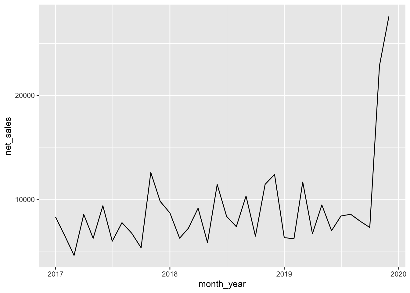
More Generalized Function
This next function is slightly more complicated as it involves creating several more columns. But it can still be generalized using the tools discussed above.
create_bpc_columns_general <- function(dataset, col_name){
    col_name <- enquo(col_name)
    bpc_data <- dataset %>%
        mutate(
            avg_orders = mean(!!(col_name)),
            # calculate lagging difference
            moving_range = diff(as.zoo(!!(col_name)), na.pad=TRUE),
            # get absolute value
            moving_range = abs(moving_range),
            # change NA to 0
            moving_range = ifelse(row_number()==1, 0, moving_range),
            avg_moving_range = mean(moving_range),
            lnpl = avg_orders - (2.66*avg_moving_range),
            lower_25 = avg_orders - (1.33*avg_moving_range),
            upper_25 = avg_orders + (1.33*avg_moving_range),
            unpl = avg_orders + (2.66*avg_moving_range)
        )

    return(bpc_data)
}

create_bpc_columns_general(net_sales_year_month_2, net_sales)
## # A tibble: 36 x 13
## net_sales Year Month Day month_year month avg_orders moving_range
## <dbl> <dbl> <chr> <dbl> <date> <dbl> <dbl> <dbl>
## 1 8284. 2017 Janu… 1 2017-01-01 1 9058. 0
## 2 6388. 2017 Febr… 1 2017-02-01 2 9058. 1896.
## 3 4589. 2017 March 1 2017-03-01 3 9058. 1798.
## 4 8533. 2017 April 1 2017-04-01 4 9058. 3944.
## 5 6237. 2017 May 1 2017-05-01 5 9058. 2295.
## 6 9370. 2017 June 1 2017-06-01 6 9058. 3132.
## 7 5959. 2017 July 1 2017-07-01 7 9058. 3410.
## 8 7740. 2017 Augu… 1 2017-08-01 8 9058. 1781.
## 9 6732. 2017 Sept… 1 2017-09-01 9 9058. 1008.
## 10 5327 2017 Octo… 1 2017-10-01 10 9058. 1405.
## # … with 26 more rows, and 5 more variables: avg_moving_range <dbl>,
## # lnpl <dbl>, lower_25 <dbl>, upper_25 <dbl>, unpl <dbl>net_sales_bpc_data <- create_bpc_columns_general(net_sales_year_month_2, net_sales)Generalized Functions for Visualization
This was the trickiest to convert into a general function and I’m still on the fence as to whether this is generalizable. In one sense, it is generalizable as I tested this create_bpc_visualization_general function on another column aside from net_sales, but it did require that I know that other columns in the dataset are: avg_orders, unpl, lnpl, upper_25 and lower_25.
I have more exploring to do around quoting and unquoting enquo(), quos() for various ggplot geometries like geom_hline. Will report back with another post once I get those details down.
create_bpc_visualization_general <- function(dataset, col_x, col_y, col_avg, col_unpl, col_lnpl, col_upper_25, col_lower_25){
    col_x <- enquo(col_x) # month_year
    col_y <- enquo(col_y) # net_sales

    col_avg <- dataset$avg_orders
    col_unpl <- dataset$unpl
    col_lnpl <- dataset$lnpl
    col_upper_25 <- dataset$upper_25
    col_lower_25 <- dataset$lower_25

    dataset %>%
        ggplot(aes(x = !!(col_x), y = !!(col_y))) +
        geom_line() +
        geom_hline(yintercept = col_avg, color = 'green') +
        geom_hline(yintercept = col_unpl, color = 'red', linetype = 'dashed') +
        geom_hline(yintercept = col_lnpl, color = 'red', linetype = 'dashed') +
        geom_hline(yintercept = col_upper_25, color = 'orange') +
        geom_hline(yintercept = col_lower_25, color = 'orange') +

        # break x-axis into quarters
        scale_x_date(breaks = '3 month') +
        # note: place before theme()
        theme_minimal() +
        theme(axis.text.x = element_text(angle = 45, hjust = 1)) +
        labs(
            title = glue('{names(dataset[,1])}: Business Process Chart'),
            subtitle = "2017 - 2019",
            x = "",
            y = glue('{names(dataset[,1])}'),
            caption = "----"
        ) +
        annotate("text", x = as.Date("2017-02-01"), y = col_unpl, color = 'red', label = "UNLP") +
        annotate("text", x = as.Date("2017-02-01"), y = col_lnpl, color = 'red', label = "LNLP") +
        annotate("text", x = as.Date("2017-02-01"), y = col_upper_25, color = 'orange', label = "Upper 25%") +
        annotate("text", x = as.Date("2017-02-01"), y = col_avg, color = 'green', label = "Avg = 97")

}

create_bpc_visualization_general(net_sales_bpc_data, month_year, net_sales, avg_orders, unpl, lnpl, upper_25, lower_25)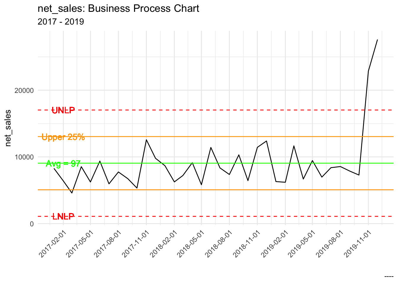
Summary
It’s possible to do a fair amount of data analysis without using functions, but functions help you avoid endless copying and pasting and make your code less error prone.
There are many different types functions you could use. In this post, I share functions that take columns of data as arguments. These types of functions are well-suited for streamlining your data pre-processing and visualization tasks.
Shout out to Bruno Rodrigues for writing Modern R with the Tidyverse which has helped me get my head around writing custom functions.